The nice thing about conditional formatting is that you have flexibility. You can base your conditions on text, dates, numbers, and even blank cells. And you choose the exact way to format it based on those rules. Here’s how to use conditional formatting in Google Sheets for everyday tasks.
Conditional Formatting For Empty Cells
Depending on the type of data you track in your spreadsheet, spotting cells that are left blank but shouldn’t be can be quite useful. And of course, there are instances when the opposite can be helpful too. A good example for using conditional formatting for empty cells is grade tracking. Whether you’re a teacher tracking test scores or a student logging your own grades, missing one can have adverse effects. Follow these steps to apply conditional formatting rules for cells that are left blank.
Give your rule and formatting a test by entering data into one of the blank cells. You should see the fill color disappear. You can also do the reverse if you have a spreadsheet that should contain empty cells and you want to spot those filled with data instead. Follow the same steps but pick Is Not Empty in the Format Cells If… drop-down box.
Conditional Formatting For Text
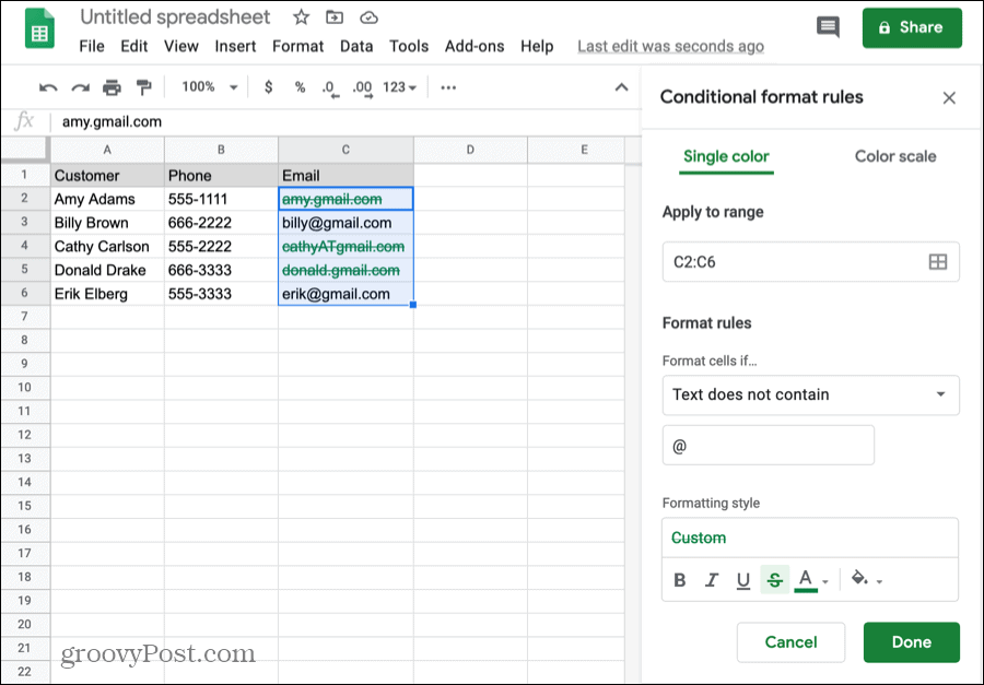
Another conditional formatting rule in Google Sheets that’s practical is for text. And you have a handful of options. You can format text that contains or does not contain, starts with, or ends with, or is exactly as the value you enter for the rule. An example you may relate to is the text that does not contain the @ (at) symbol for email addresses. You might receive a data dump that has customer or client email addresses. Before you set up a mail merge, you’ll need to remove those addresses that are invalid; they do not contain the @ (at) symbol.
Using text rules for conditional formatting gives you tons of options. Just pick the one that applies to your particular spreadsheet in the Format Cells If… drop-down box.
Conditional Formatting For Dates
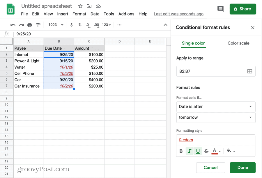
One common piece of information in many spreadsheets is the date. And that’s why this conditional formatting rule is a popular one. Automatically format text based on an exact date, one before another, or one after another. A terrific use for this rule is home budgeting and/or bill tracking. If you keep a spreadsheet for your monthly budget with due dates for bills, you can quickly see those you have coming up. Here, you’ll use the Date Is After condition.
Now each time you open this spreadsheet, bills with due dates after tomorrow (or today if you prefer) will jump right out so you can prepare or pay them. You can look at the other date rules available for different situations. And, check out our tutorial to create a calendar in Google Sheets for another date-related feature.
Conditional Formatting For Numbers
If there’s anything more common in a spreadsheet than a date, it’s a number. Whether it’s a standard number, currency, percentage, or decimal, you will likely find it in a spreadsheet. One thing many people use spreadsheets for these days is weight tracking. Maybe you do too and log your weight each day or week. And if so, you probably have a goal for the weight or a range you want to stay within. Or perhaps you track your calorie intake and want to keep an eye on those numbers. For simplicity, we’ll use formatting to show weight in pounds above a certain number.
And be sure to keep the other number rules for conditional formatting in mind: greater than or equal to, less than or less than or equal to, is equal to or not equal to, and is between or not between.
Spot Your Data At a Glance in Google Sheets
With conditional formatting in Google Sheets, you can quickly and easily spot the data you need at a glance. You don’t have to search, sort, or filter your sheet to see important data. Conditional formatting in Excel may feel a bit more robust, but the options in Google Sheets may be exactly what you need. And if you’d like help with that final rule you see in the Format Rules drop-down box for Custom Formula Is, take a look at our example use for highlighting duplicates in Google Sheets.


![]()
